Computational and Asymptotic Complexity

• Algorithms are an essential aspect of data structures.
• Data structures are implemented using algorithms.
• Some algorithms are more efficient than others.
• Efficiency is preferred; we need metrics to compare them.
• An algorithm’s complexity is a function describing the efficiency of the algorithm in terms of the amount of data the algorithm must process.
• Time complexity is a measure of how long the function takes to run in terms of its computational steps.
• Space complexity has to do with the amount of memory used by the function.
• Efficiency covers various resources, including CPU (time) usage, memory usage, disk usage, and network usage.

Differentiating Between Performance and Complexity

• Performance: How much time/memory/disk/… is actually used when a program is run. This depends on the machine, compiler, etc. as well as the code.
• Complexity: How do the resource requirements of a program or algorithm scale, i.e., what happens as the size of the problem being solved gets larger?
• Complexity affects performance but not the other way around.

Big-O Notation

• Big O notation is used in Computer Science to describe the performance or complexity of an algorithm and measure the algorithm’s efficiency.
• It measures the time it takes to run the function as the input grows and can be used to describe the execution time required or the space used (e.g., in memory or on disk) by an algorithm.
• Big O is sometimes referred to as the algorithm’s upper bound, dealing with the worst-case scenario.

How to Determine Complexities

• Ignore constant factors, e.g., 6n -> we read as O(n).

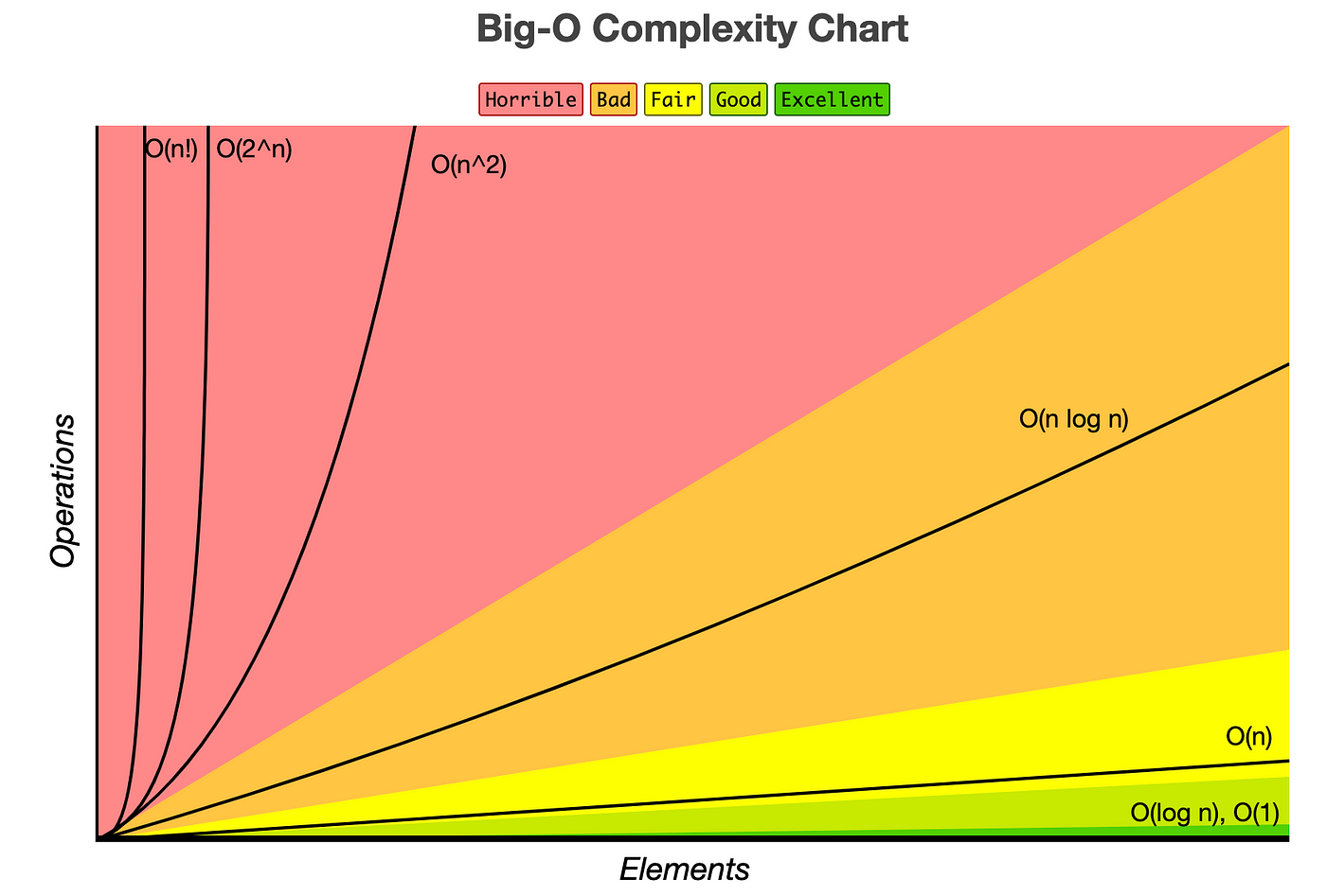
• Certain terms “dominate” others, so ignore low-order terms, e.g., O(1) < O(log n) < O(n) < O(n log n) < O(n^2) < O(2^n) < O(n!).

• When writing Big O notation, look for the fastest-growing term as the input gets larger and larger. You can simplify the equation by dropping constants and any non-dominant terms.
• For example, O(2^N) becomes O(N), and O(N² + N + 1000) becomes O(N²).

Common Big-O Functions

O(1) Constant Time

• Constant time algorithms always take the same amount of time to be executed.
• The execution time of these algorithms is independent of the size of the input.
• Examples include accessing an array element by index, inserting a node into a linked list, pushing and popping from a stack, enqueuing and dequeuing from a queue, and arithmetic operations (e.g., addition, subtraction, multiplication, division, etc.).
• Asigning a value to a variable
• Inserting a element in an array

O(n) Linear Time

• Linear time algorithms take time that is directly proportional to the size of their input, n.
• If the problem size doubles, the number of operations also doubles.
• Example: Traversing data or elements in a vector using an iterator.

O(n²) Quadratic Time

• Quadratic time complexity.
• Example: Nested loops where the inner loop executes n times for each execution of the outer loop. The complexity is O(n²).

O(log n) Logarithmic Time

• Logarithmic time complexity.
• Algorithms with this complexity grow slower as n grows.
• Examples include binary search and certain sorting algorithms like quicksort.
• Logarithmic time can be identified when the counting variable doubles instead of incrementing by 1.

Understanding Big O notation is important in writing algorithms. It helps you determine when your algorithm is getting faster or slower and allows you to compare different methods to choose the most efficient one.